Sampling Error

Bias as a statistical term means error. To say that you want an unbiased sample may sound like you're trying to get a sample that is error-free. As appealing as this notion may be, it is impossible to achieve! Error always occurs -- even when using the most unbiased sampling techniques. One source of error is caused by the act of sampling itself. To understand it, consider the following example.

Let's say you have a bowl containing ten slips of paper. On each slip is printed a number, one through ten. This is your "population." Now you are going to select a sample. We will use a random method for drawing the sample, which can be done easily by closing your eyes and reaching into the bowl and choosing one slip of paper. After choosing it, check the number on it and place it in the sample pile.

Now to determine if the sample is representative of the population, we must know what attribute(s) we wish to make representative. Since there are an infinite number of human attributes, we must precisely determine the one(s) we are interested in before choosing the sample.

In our example, the attribute of interest will be the average numerical value on the slips of paper. Since the "population" contained ten slips numbered consecutively from one to ten, the average numerical value in the population is:

On our second pick, we choose a slip that has a 1 on it. Now the mean of sample values is:

• larger than the population mean,
• smaller than the population mean, or
• equal to the population mean

Theoretically, each sampling causes the sample mean to approach a bit closer to the population mean. In effect, the sampling error progressively declines as the sample size increases.  Although we can never know for certain what the sampling error curve looks like (because by definition we do not know what the true population mean is of the attribute we're sampling), we can estimate that the shape of the error curve is similar to that of a damped harmonic oscillation.  See the figure below.

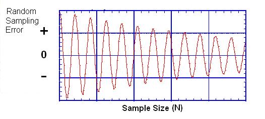
This figure suggests two interesting things.  First, it suggests that the error generated by a random sampling of subjects from a population is cyclic and predictable:  it steadily decreases in amplitude (size) as the number of subjects sampled from the population increases. Second, the error curve suggests that it can be mathematically modeled.  This is particularly important.  Because a basic function of parametric statistics is to estimate the amount sampling error produced by a sample of a given size.  The only way such an estimate can be reliably calculated is if the error curve, itself, is a predictable shape and decreases at a predictable rate.

Eventually, if we sampled everyone from the population, the sample mean and the population mean would become equal.  Another way of saying this is that the sampling error would decrease to 0. This is why a complete population census is completely accurate -- there is no sampling error.

However, researchers are usually compelled by logistical, time, and money reasons to use a relatively small portion (sample) of a population. The general rule is that the larger the sample the less sampling error there will be, and the more confident the researcher can be that the sample is representative of the population from which it was drawn.

Equally important to the size of the sample is the determination of the type of sampling to be done. In our example, we randomly (blindly) chose from the population. Random sampling always produces the smallest possible sampling error. In a very real sense, the size of the sampling error in a random sample is affected only by random chance. The two most useful random sampling techniques are simple random and stratified random sampling methods. These will discussed shortly.

Because a random sample contains the least amount of sampling error, we may say that it is an unbiased sample. Note that we are not saying the sample contains no error, but rather the minimum possible amount of error.

Nonrandom sampling techniques also exist, and are used more frequently than you might imagine. As you can probably guess from our previous discussion, nonrandom sampling techniques will always produce larger sampling errors (for the same sample size) than random techniques. The reason for this is that nonrandom techniques generate the expected random sampling error on each selection plus additional error related to the nonrandom nature of the selection process. To explain this, let's extend our sampling example from above.

Let's say we want to sample from a "population" of 1000 consecutively numbered slips of paper. Because numbering these slips is time consuming, we have 10 people each number 100 slips and place all 100 of them into our bowl when they finish. Let's also say that the last person to finish has slips numbered from 901 to 1000, and these are laid on top of all the other slips in the bowl. Now we are ready to select them.

If we wanted to make this a truly random sampling process, we would have to mix the slips in the bowl thoroughly before selecting. Furthermore, we would want to reach into the bowl to different depths on subsequent picks to make sure every slip had a fair chance of being picked.

But, let us say in this example that we forget to mix the slips in the bowl. Let's also say we only pick from the top layer of slips. It should be obvious what will occur. Any sample (of 100 or less) we select from the top layer of slips (numbered 901 through 1000) will generate a mean somewhere around 950.5 (the true mean of the numbers 901 through 1000). Clearly, this is not even close to the true population mean (500.5 -- the mean of the numbers from 1 to 1000). In this example, the sampling error would be somewhere around 450 (950.5 - 500.5)--a mighty large sampling error!

This was a simple, and somewhat absurd, example of nonrandom sampling. But, it makes the point that nonrandom sampling methods generate more sampling error (bias) than random sampling methods, and produce samples that are usually NOT representative of the general population from which they were drawn.

Nonrandom sampling methods do not generate a predictable error curve.  In fact, the error curve for a nonrandom sample could be very erratic.  This is the primary reason why nonrandom sampling methods are not desirable (although they are sometimes the only way to generate a sample for a particular research study).  Since the error curve can not be predicted in terms of its shape or the rate at which it decreases, it's impossible to accurately estimate the amount of sampling error generated by a sample of any size (less than the entire population).  That why we say that random sampling methods always produce less sampling error than a nonrandom method for the same sample size.

Bottom line: random sampling methods are preferred over nonrandom sampling methods.